Learning the regulatory code of the genome using Basset
Convolutional neural networks are widely used to understand the DNA sequence of data. In this blog, we will be discussing about one such model (Basset model) along with its implementation.
Origin:
Though we know that, most of the diseases comprise of non-coding variants, the mechanisms behind these variants are not known. Here, we address this challenge using a recent machine learning advance - deep convolutional neural networks (CNNs). We have developed a model, Basset to apply CNNs to learn the functional activity of DNA sequences from genomics data.
Our model Basset has certain characteristics which are termed systematically:
i.study the cell-specific regulatory code of the chromatin accessibility
ii. clarify the concept learned by the model.
Thus, Basset provides a powerful computational approach to clarify and elucidate the non-coding genome.
Synopsis:
To learn the DNA sequence signals of open versus closed chromatin in these cells, we apply a deep CNN. CNN’s perform adaptive attribute extraction to map input data to informative representations during training.
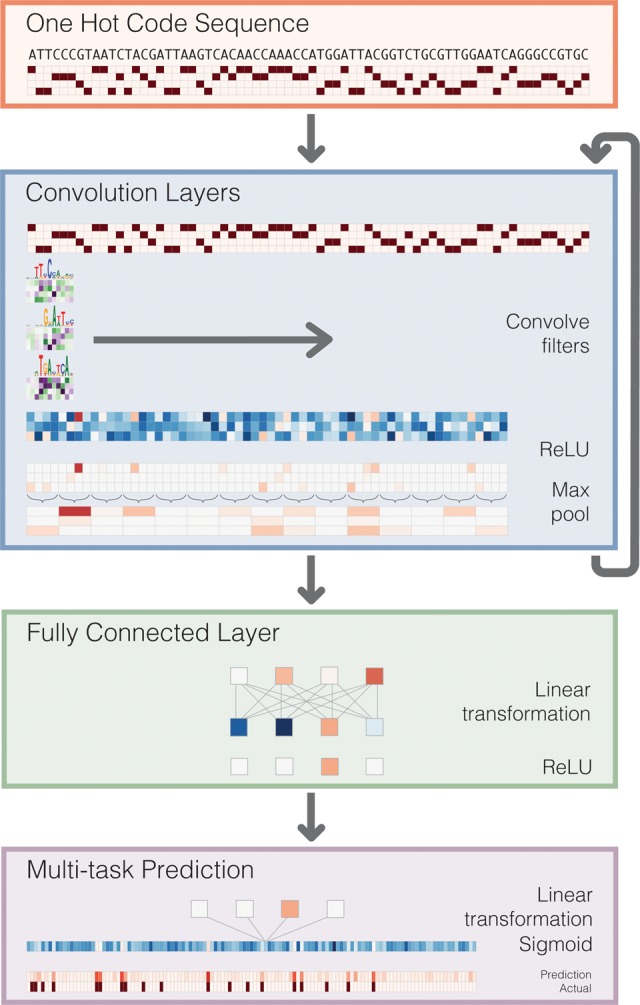
Convolution layers:
The first convolution layer operates directly on the one-hot coding of the input sequence of length 600 bp. It optimizes the weights of the set of position weight matrices (PWMs). These PWM filters search for the relevant patterns along the sequence and output a matrix with a row for every filter and a column for every position in the sequence. And the subsequent convolution layers consider the orientations and spatial distances between patterns recognized in the previous layer.
We apply a ReLU activation function after each convolution layer to obtain a more expressive model. This is done since computing non-linear functions of the information flowing through the network give more expressive models.
Then we perform the Max Pooling. It reduces the dimension of the input and so the computation in the next layers also decreases. It also provides in-variance to small sequence shifts to the left or right. In short, even if the sequence is slightly shifted to the left or right the model remains independent of this behavior.
Fully Connected Layers:
Fully connected layers perform a linear transformation of the input vector and apply a ReLU.
Prediction layer:
The output of the fully connected layers is fed as input to the final layer and the Sigmoid activation is applied.The final layer outputs 164 predictions for the probability that the sequence is accessible in each of the 164 cell types.
The full architecture of our neural network consists of three convolution layers and two are completely layers of fully connected hidden nodes.
Implementation:
I. Data Preprocessing:
i) First, the DNA sequences are given in the fasta file.
ii) So, our first task would be to perform one-hot encoding of these DNA sequences.
from sklearn.preprocessing import OneHotEncoder
from sklearn.preprocessing import LabelEncoder
import numpy as np
import torch
import re
def string_to_array(my_string):
    my_string = my_string.lower()
    my_string = re.sub('[^acgt]', 'z', my_string)
    my_array = np.array(list(my_string))
    return my_array

label_encoder = LabelEncoder()
label_encoder.fit(np.array(['a','c','g','t','z']))
def one_hot_encoder(my_array):
    integer_encoded = label_encoder.transform(my_array)
    onehot_encoder = OneHotEncoder(sparse=False, dtype= int, n_values=5)
    integer_encoded = integer_encoded.reshape(len(integer_encoded), 1)
    onehot_encoded = onehot_encoder.fit_transform(integer_encoded)
    onehot_encoded = np.delete(onehot_encoded, -1, 1)
    return onehot_encoded
II. Well defined Model Architecture:
Here we define the model as Basset with three convolution layers and two layers of fully connected hidden nodes. We have even performed Batch normalization for scaling the activations after each convolution layer. The same thing we have also done before the activation layer.
def get_model(load_weights = True):
    Basset= nn.Sequential( # Sequential,
        nn.Conv2d(4,300,(19, 1)),
        nn.BatchNorm2d(300),
        nn.ReLU(),
        nn.MaxPool2d((3, 1),(3, 1)),
        nn.Conv2d(300,200,(11, 1)),
        nn.BatchNorm2d(200),
        nn.ReLU(),
        nn.MaxPool2d((4, 1),(4, 1)),
        nn.Conv2d(200,200,(7, 1)),
        nn.BatchNorm2d(200),
        nn.ReLU(),
        nn.MaxPool2d((4, 1),(4, 1)),
        Lambda(lambda x: x.view(x.size(0),-1)), # Reshape,
        nn.Sequential(Lambda(lambda x: x.view(1,-1) if 1==len(x.size()) else x ),nn.Linear(2000,1000)), # Linear,
        nn.BatchNorm1d(1000,1e-05,0.1,True),#BatchNorm1d,
        nn.ReLU(),
        nn.Dropout(0.3),
        nn.Sequential(Lambda(lambda x: x.view(1,-1) if 1==len(x.size()) else x ),nn.Linear(1000,1000)), # Linear,
        nn.BatchNorm1d(1000,1e-05,0.1,True),#BatchNorm1d,
        nn.ReLU(),
        nn.Dropout(0.3),
        nn.Sequential(Lambda(lambda x: x.view(1,-1) if 1==len(x.size()) else x ),nn.Linear(1000,164)), # Linear,
        nn.Sigmoid(),)
III.Training:
This model is trained on the DNA-seq data sets of 164 cell types which is found in the Road Map and ENCODE Consortium.
IV. Testing:
For testing, we provide the model with a sample sequence of length 600bp the .The model is also known to make predictions for the DNA accessibility of 164 cell-types.
test_sequence='TTTGTGGGAGACTATTCCTCCCATCTGCAACAGCTGCCCCTGCTGACTGCCCTTCTCTCCTCCCTCTCGCCTCAGGTCCAGTCTCTAAAAATATCTCAGGAGGCTGCAGTGGCTGACCATTGCCTTGGACCGCTCTTGGCAGTCGAAGAAGATTCTCCTGTCAGTTTGAGCTGGGTGAGCTTAGAGAGGAAAGCTCCACTATGGCTCCCAAACCAGGAAGGAGCCATAGCCCAGGCAGGAGGGCTGAGGACCTCTGGTGGCGGCCCAGGGCTTCCAGCATGTGCCCTAGGGGAAGCAGGGGCCAGCTGGCAAGAGCAGGGGGTGGGCAGAAAGCACCCGGTGGACTCAGGGCTGGAGGGGAGGAGGCGATCCCAGAGAAACAGGTCAGCTGGGAGCTTCTGCCCCCACTGCCTAGGGACCAACAGGGGCAGGAGGCAGTCACTGACCCCGAGACGTTTGCATCCTGCACAGCTAGAGATCCTTTATTAAAAGCACACTGTTGGTTTCTGCTCAGTTCTTTATTGATTGGTGTGCCGTTTTCTCTGGAAGCCTCTTAAGAACACAGTGGCGCAGGCTGGGTGGAGCCGTCCCCCCATGGAG'
numpy_ex_array=one_hot_encoder(string_to_array(test_sequence))
shape = numpy_ex_array.shape
temp = np.reshape(numpy_ex_array,(1,shape[1],shape[0],1))
torch_ex_float_tensor = torch.from_numpy(temp)
torch_ex_float_tensor=torch_ex_float_tensor.float()
model = get_model(load_weights = True)
model=model.cpu()
#print(model)
out=model(torch_ex_float_tensor)
print(out)
Here, first wee need to one-hot encode the test sequence and then reshape the numpy array. Thus it becomes compatible with the shape of the input for the model and feeds it to the model. It thus makes room for the model on making predictions of the DNA accessibility.
Summary:
Given an SNP pair, by these predicted chromatin accessibility values, we can calculate the difference between the accessibilities of the variants in the two alleles. The difference can be ranked which could be useful for predicting the causal variants.