All you need to know about Variational AutoEncoder
Variational AutoEncoders are being widely used in generative models since the day they came into existence. This blog is just a synopsis of understanding Variational AutoEncoders.
Vae is a generative model which helps us to generate a similar type of input data. It helps to generate similar images, similar text, etc.
A generative model is a way of learning data distribution of input data so that it produces a new similar data.
VAEs also makes a probability distribution of input data, and from that distribution, we create samples which are taking data from this distribution and generate new data similar to input data.
In this blog we are going to learn about:
- Encoder
- Latent_vector(sample vector)
- Decoder
- Goal of VAE
- Loss Function in VAE
- Optimization
- Reparameterization
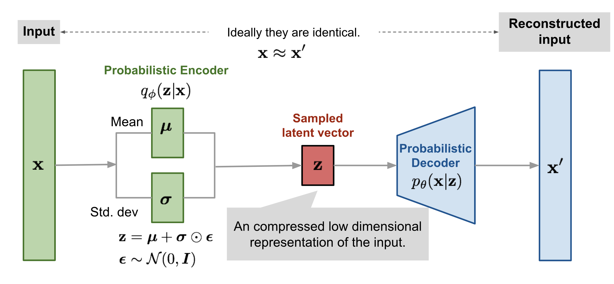
So as we see in the above diagram, Vae has mainly given importance on 3 components or states we divide the VAE into three parts for better understanding.
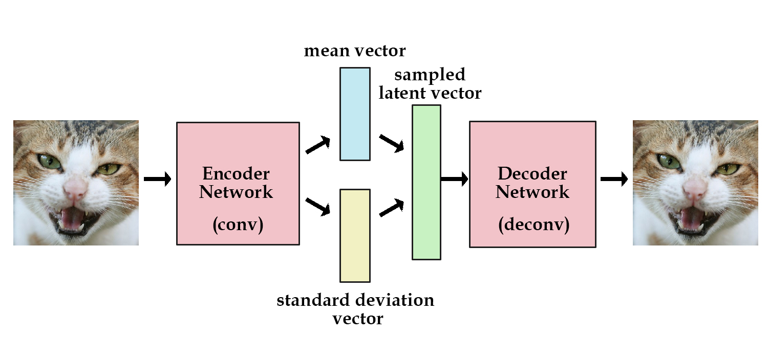
Encoder: Encoder is a neural network that takes input data, converts higher dimensional data into lower dimensional data also known as latent space. Let’s say we have an image of 28*28(784) pixels, what we as encoder do is convert our 784-dimensional images into a small dimension of 8. The encoder basically tries to pass information of whole 784 dimension images into 8 dimension vector. It is encoded in such a way that the whole 8-dimensional space looks like the whole input data.
In Vae we do not say encoder, we say probabilistic encoder. This is a typical thing which is used in Vae and most of the people are aware of that. It is done because the small dimensional latent space does not take a discrete range of values. It only takes the probability distribution. As stated above, we have an 8-dimensional small vector then 8 nodes represent some character of input data. e.g. if our input data is faces of human, then these nodes may represent smiles, eye shape, etc and create a probability distribution of these characters.
We represent encoder as $q_\phi(z|x)$ which means find the z(small dimension latent space) given x which is input data. In general case, we take $q_\phi(z|x)$ is Gaussian distribution you can take any distribution whose distribution you know. But since it is not so important, we will flourish on it later.

Latent Space: It is a layer in the neural network which represent our whole input data. It is also called bottleneck because of in very small dimension it represents whole data.
Decoder: From the below diagram you will understand what is the role of the decoder in VAE. It converts the latent sample space back to our input data. It also has the ability to convert our 8-dimensional latent space into the 784-dimensional image.
We represent decoder as $p_\theta(x|z)$ which means to find x provided z.
Objective of Vae
The main purpose of VAE is to find gaussian distribution $q_\phi(z|x)$ and take a sample from z ~ $q_\phi(z|x)$ (sampling z from $q_\phi(z|x)$) and generate almost identical output.
Importance of Gaussian in VAE encoder
You may notice in encoder section that we use Gaussian distribution. But first, you need to have a clear idea, why we take a known distribution in encoder region.
Let x be the input and z be the set of latent variables with joint distribution $p(z,x)$ the problem is to compute the conditional distribution of z given x $p(z|x)$.
To compute $p(z\mid x)=\frac{p(x\mid z)\, p(z)}{p(x)}$ we have to compute the $p(x)=\int_{z} p(x,z) dx$ but the integral is not available in closed form or is intractable(i.e require exponential time to compute) because of multiple variable involved in latent vector z.
To get away with this problem we use an alternative solution. We actually approximate $p(z\mid x)$ with some known distribution $q(z\mid x)$ that is tractable. This is done by Variational Inference(VI) We use KL-divergence to approximate the $p(z\mid x)$ and $q(z\mid x)$.This divergence measures how much information goes off-track while using q to represent p. It is one measure q close to p and we try to minimize the KL-divergence in order to get similar distribution.
Points to remember about KL-divergence:
- It is always greater than 0
- $D_{kl}(q_\phi(z\mid x)||p_\theta(z\mid x))\neq D_{kl}(p_\theta(z\mid x)||q_\phi(z\mid x))$
Loss Functions in VAE: We have to minimise two things. One is kl-divergence so that one distribution similar to another and other is a reconstruction of input back from latent vector as we see latent vector is very less dimension as compared to input data, so some details is lost in converting back data. To minimise this loss, we use reconstruction loss. This loss function tells us how effectively the decoder decoded from z to input data x.
As we see, we have two loss function one for reconstruction loss, and other is divergence loss. This loss function is known as variational lower bound or evidences lower bound.
This lower bound comes from the fact that KL-divergence is always non-negative. Through minimizing the loss, we are maximizing the lower bound of the probability of generating new samples.
Optimization
When we want to minimize the loss function $min_{\theta,\phi}L(\theta,\phi)$ here $\theta$, $\phi$ are learnable parameters also say weights and biases terms. This is done by differentiating one parameter at a time. We can learn one parameter and keep another parameter constant and find the minimum value. Then put this minimum value into the second differentiable parameter. By doing this, you minimize the loss after various repetition. Hence the main problem with minimizing the loss is to differentiate the $\phi$ term because $\phi$ appears in the distribution from which expectation is taken if you observe above loss you see z is taken from $q_\phi(z\mid x)$.
Reparameterization When we implement encoder and decoder in the neural network, we need to backpropagate through random samples. Backpropagation cannot flow through the random node. In order to overcome this obstacle, we use reparameterization trick. Instead of sampling from $z\sim q_\phi(z\mid x)$ we sample from N(0,1) i.e $\epsilon \sim N(0,1)$ then linear transform using $z=\mu+\sigma⊙\epsilon$
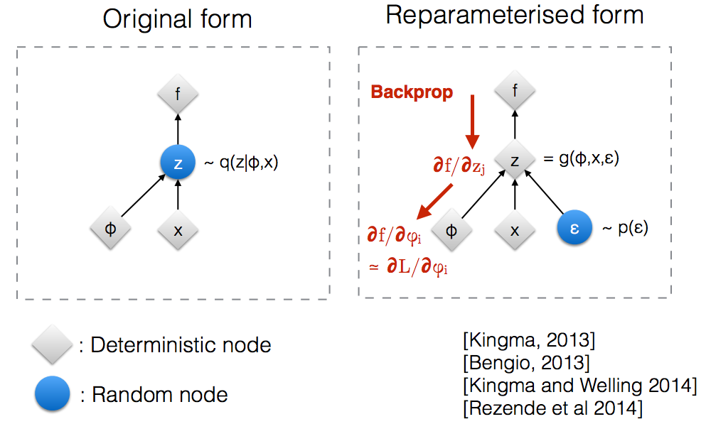
The reparametrization consists of saying that sampling from $z\sim N(\mu,\sigma)$ is equivalent to sampling $\epsilon∼N(0,1)$ and setting $z=\mu+\sigma⊙\epsilon$. After reparametrization we easily backpropogate.
So that’s the end of the theory section. I hope you like it and in the next part, we will implement the VAE for a molecular generation or the text generation where we use molecules as SMILES.
References
From Autoencoder to Beta-VAE and Variational Autoencoders Explained nice explanation in these blogs I used images from these blogs
Alhad Kumar this youtube channel by alhad Kumar explain VAE concepts easily.